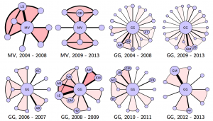
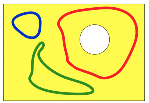
Network comparison: Distance and Homology

Data is getting big, but more than big it is getting pervasive. As our lives become more dependent and integrated with the digital infrastructure, more aspects of our life get measured and recorded. This pervasiveness leads to the emergence of novel types of signals for which existing analytic tools cannot be applied easily. Networked data falls in this category. As an example, the networks above are the co-authorship networks constructed from IEEE Transaction on Signal Processing publications of two famous signal processing researchers, Prof. Georgios B. Giannakis (GG) of the University of Minnesota and Prof. Martin Vetterli (MV) of the École Polytechnique Fédérale de Lausannee for the selected timeframe. Each node in the networks represents an author. The size of the nodes is proportional to the number of publications of the corresponding authors. The width of the links is proportional to the number of publications between the author pairs. Color intensity of the shading triangles is proportional to the number of publications to the enclosed author triplets. Distinguishable differences exist in their respective collaboration patterns. A natural question is: how can we quantify the differences between high order networks?

Such a problem has been solved by comparing some features of the respective networks. Feature analysis is application dependent, utilizes only a small portion of the information conveyed, and may yield conflicting judgments — two networks close to each other are quiet different from the third. For the networks presented above, it is not clear which features one should use. Moreover, feature analysis is not easily generalizable to incorporate high dimensional information, e.g. publications between three or four authors, as what we did in the example. We tackle this problem from a different perspective — by defining valid metric distances, which are universal, depend on all edge weights, and are null if and only if the networks are isomorphic. We also establish a connection between Network Science and Computational Topology and uses tools from the latter to efficiently quantify network differences.

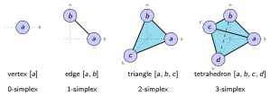
In specific, besides relationship between pairs of nodes, we also consider high order relationships between three nodes or four nodes. Such consideration is meaningful in practice, because the collaboration between three authors is different from the collaboration between two authors, and collaboration between four authors is not the same as the collaboration between two authors. Formally, we consider high order networks of order $K$ as a tuple $N_X^K = (X, r_X^0, r_X^1, \dots, r_X^K)$, where $X$ is the set of nodes, and $r_X^k$ is a mapping from $k+1$ tuples to $\mathbb{R}_+$ quantifying the relationship between $k+1$ elements in $X$. We require that the relationship $r_X^2(A, B, B)$ between $A$, $B$, and $B$ to be the same as the relationship $r_X^1(A, B)$ between $A$ and $B$. In common scenarios, relationship either quantifies the similarity or the dissimilarity between tuples. When it denotes proximities, we require $r_X^2(A, B, C) \leq r_X^1(A, B)$; when relationship functions represent dissimilarity, we require $r_X^2(A, B, C) \geq r_X^1(A, B)$.

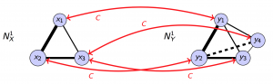
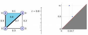
Because we need to measure the dissimilarity between networks of arbitrary sizes, we need a way to map nodes between networks with different number of nodes. We use a mathematical tool called correspondence. A correspondence $C$ between two set of nodes $X$ and $Y$ is a subset of $X \times Y$ such that for any $x \in X$, there exists $y \in Y$ with $(x, y) \in C$, and for any $y \in Y$, there exists $x \in X$ with $(x, y) \in C$. This is a generalization of permutation and enables us to map node sets with different cardinality. Given a pair of networks $N_X^K$ and $N_Y^K$, and a specific correspondence $C$, the difference between the two networks measured by the correspondence can be defined as the bottleneck tuple where the respective relationship functions is the most different
\begin{align}
\Gamma_{X, Y}^k (C) = \max_{(x_{0:k}, y_{0:k}) \in C} \left\| r_X^k(x_{0:k} – r_Y^k(y_{0:k}))\right\|.
\end{align}

The network distance between the pair of networks for the $k$-th order can then be defined by searching for the correspondence that makes the networks the most similar,
\begin{align}
d_{\mathcal{N}}^k (N_X^K, N_Y^K) = \min_{C \in \mathcal{C}(X, Y)} \left\{ \Gamma_{X, Y}^k (C) \right\}.
\end{align}

This network distance works well in distinguishing the collaboration pattern of different researchers. The figure above shows the multi-dimensional scaling of the distance between the networks shown in the introductory paragraphs, where the networks from Prof. Martin Vetterli is shown in red, the 2-year networks from Prof. Georgios Giannakis is in black, and the 5-year networks from Prof. Georgios Giannakis is in blue.

Network distances are useful tools; however, since we need to evaluate all possible choices of correspondence, the exact network distance is hard to evaluate when networks are large. Therefore, we would like to find tight approximations of the network distance. This is achieved through persistent homology tools from computational topology. The building block in topology is simplex, which is just the convex set of several points.

With simplices, we could construct simplicial complex, which is a collection of simplices that are glued together.

An important concept about simplicial complex is homology, which describe holes that do not have interiors. As an example, consider three rubber bands in a two-dimensional plane where only the red rubber band encloses a hole. Imagine yourself able to move the bands arbitrarily in the plane however cannot lift them from the plane. Then, no matter how you move them, only the red rubber band will enclose the hole. Homological features are defined to formalize this notion. In the simplicial complex above, $[a, b]$, $[b, d]$, $[d, a]$ form a cycle; however, there is an interior formed by $[a, b, d]$, and therefore, this hole is not a homological feature. Simultaneously, $[b, c]$, $[c, d]$, $[d, b]$ form a cycle, and there is not interior between them; therefore, this hole is a homological feature.

Homology is useful, however, there is no way for us to incorporate weights. To do that, we introduce an artificial dimension — time, and assign each simplex a value corresponding to its relationship function representing when does the simplex appears. As the dummy time increases, more and more simplices get included in the filtration. Persistent homology then records the changes in homological features with the filtration of simplices. As an example, there is one homological features between time 0.7 and 0.8, and there is another homological feature that is born at 0.5 and stays there forever. The plot on the right shown above is named persistence diagram.

To quantify the difference in persistence diagrams, we find the best mapping between the points in the persistence diagram, and use the difference that cannot be matched well in the best mapping as the difference between the persistence diagrams.

When the two persistence diagrams have different number of points, we can consider the persistence diagram with smaller number of points actually possesses a number of points that are on the diagonal. Therefore, each point in the persistence diagram may be mapped to an actual point in the other persistence diagram, or mapped to the point on the diagonal in the other persistence diagram which yields the smallest discrepancy. Our main result in this track of research is that difference between persistence diagram is a tight lower bounds of the network distance. If the networks are constructed carefully, not much information is lost in the corresponding persistence diagram, and there are practical scenarios where the lower bound is the same as the actual network distance.

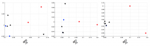
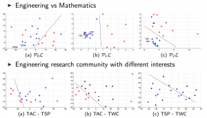
We applied these homological lower bounds to distinguish networks constructed from publications in different journals, e.g. engineering and mathematics. We found that the network lower bounds could successfully distinguish the research patterns in different communities. We also considered a more challenging task, to distinguish networks from engineering research communities with different interest, e.g. signal processing, automatic control, and wireless communication. These homological tools made a moderate success in classifying them as well.

Network comparison: Distance and Homology